Risk, Measured — Bayesian Risk Analysis on the Live Mine Plan

A mine plan’s headline NPV is built from dozens of guesses — the copper price in 2038, the grade of ore not yet adequately drilled, the capital cost of a plant nobody has built. The industry knows this, and the better operators are already moving: probability-weighted cases, P-ranges on reserves, risk-adjusted hurdle rates. The direction of travel is clear. The execution, mostly, is not.

Because behind most “probabilistic” studies still sits the same machinery: a tornado chart flexing one guess at a time by a ±15% that was itself a guess; a Monte Carlo bolted onto a single frozen cash-flow line; distributions asserted rather than derived, with every metal shocked in lockstep and the plan standing conveniently still. The ambition is right. The substrate can’t deliver it.

This paper describes what delivering it actually takes — and is precise about a word that gets abused along the way: Bayesian.

1. What we mean by Bayesian

The word has a precise meaning: you state a prior belief, confront it with data through a likelihood, and get a posterior — a belief disciplined by evidence. No data, no update, no posterior. It’s a high bar, and it isn’t met everywhere in our own system — so here is the taxonomy, stated plainly:

Where data exists, we update. Where the deposit is the data, we measure. Where no data exists, we say so — and propagate your stated judgment honestly instead of dressing it up in statistics it doesn’t have.

2. Price: judgment, disciplined by the market

A price assumption over a 20-year mine life is not one number — it’s a process: where does the price settle, how fast do shocks decay, how violent is the ride. Our calibration treats each of those as a parameter with a prior your team states in plain terms, then confronts them with three kinds of evidence:

• The forward curve — the market’s own tradeable expectation, the strongest signal on the path ahead;
• Decades of real price history — which informs dynamics only: how volatile the metal is and how fast shocks fade. Thirty-year-old prices know how copper moves; they know nothing about where a structurally different market settles, and the model is built so they can’t vote on it;
• Realised volatility from recent trading.

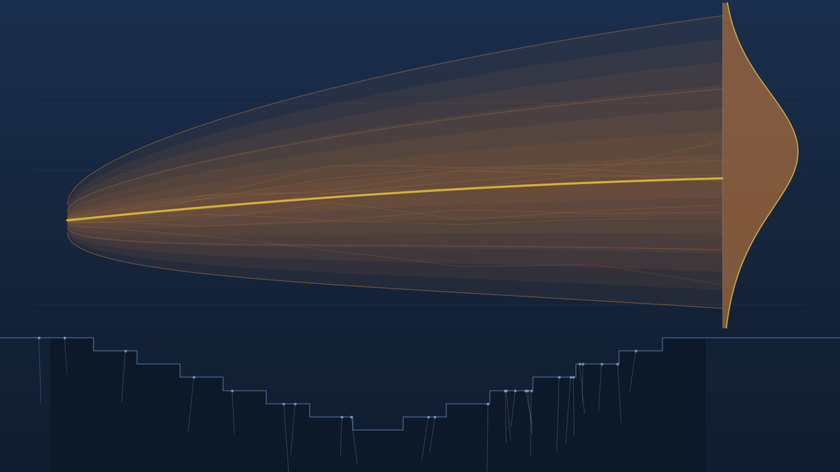
The output is a price cone, not a flex: tight in near years where the strip pins it down, widening with horizon, asymmetric the way lognormal prices actually are. And every parameter carries a provenance receipt — how much of the posterior came from data, how much stayed with your judgment:

Share of each posterior parameter driven by market data on a copper calibration. The market knows volatility; nobody’s data knows the 2040 price — so the level stays with the people paid to have a view. The system shows you the boundary instead of hiding it.

And when the house view and the market disagree, the system doesn’t pick a winner silently. Run the risk on your basis — the cone re-anchored to your deck price — and the calibration still reports, alongside it, the market-implied probability of that deck being achieved. Our view: that number belongs on the IC slide, not buried. “Here is our basis, here is the risk around it, and here is what the market implies about our basis” is the most credible sentence a proponent can say.

3. Polymetallic projects: stop shocking gold with a copper price

Most copper projects aren’t copper projects — they’re copper-gold-silver-byproduct projects. Yet nearly every risk tool applies one price flex to total revenue, which quietly assumes every metal crashes and rallies in lockstep with the primary. That erases the single most valuable feature of a polymetallic asset: gold is counter-cyclical. In precisely the scenarios your downside percentile cares about — recession, copper collapsing — gold historically holds or rises. A Cu-Au orebody carries a built-in hedge, and single-price risk models destroy it on contact.

Our engine prices each element with its own calibrated cone, correlates them realistically (copper-gold correlation is weak, and you control it), and blends them with revenue weights derived from the actual mine schedule, year by year — because the gold share of revenue in year 14 is not what it was in year 2, and the schedule already knows that. On a copper-gold development in our database, correcting this one error moved the downside percentile of NPV by roughly half a billion dollars. Not because the project changed — because the model stopped destroying a hedge the orebody actually owns.

The same discipline runs through the cost side: treatment and refining charges are volume-linked ($/t of concentrate, ¢/lb of payable metal), so when a price scenario crashes, TC/RC correctly stays put and squeezes the netback — instead of conveniently shrinking with revenue, as flexed models silently assume. And the derivation of those charges is validated line-by-line against the plan’s own cost build, with the fidelity of every component reported before anyone trusts it.

4. Grade: measured from your drilling, not assumed

Grade risk is where the industry’s conventions are least well informed by actual data: a flat ±10% flex, applied identically to year 1 (grade-controlled, drilled at 25-metre spacing) and year 18 (inferred material barely touched). Serious research is closing this gap — conditional simulation and the stochastic mine planning work built on it, with McGill’s COSMO laboratory prominent among the leaders — but those methods remain data- and specialist-intensive. Our approach is a ladder — each rung shipped, each labelled by where its numbers come from.

Tier one builds a grade cone from the schedule’s own resource-classification mix — each year’s feed is a known blend of measured, indicated and inferred material, so each year gets an uncertainty reflecting the drilling maturity of what’s actually being mined that year: tight early, wide late.

Tier two goes further — it asks the deposit itself. Where drill holes are loaded, the system removes each hole and re-estimates it from its neighbours — thousands of blind predictions scored against reality. That yields the orebody’s own spacing-versus-confidence curve, its own error-correlation range, and — after accounting for how errors average out across a year’s mill feed — its own annual grade risk, per resource class.

On that same copper-gold project, the measured envelope came out at roughly half the industry-convention bands — annual grade risk of ~3% where convention assumes 6–10%. A well-drilled disseminated deposit’s block-scale noise cancels hard across thirteen million tonnes of annual feed, and now that’s a demonstrated property of this orebody, not an analyst’s assertion.

Tier three closes the loop with the plan itself. The pit optimiser and scheduler already flag every block with the period it is mined. Linking those flags to the measured error field makes grade risk spatial: each year’s uncertainty is evaluated where that year’s mining actually happens — the local drill spacing of the mined panels, aggregated over that year’s real footprint using the correlation range measured from the drilling. Even the correlation between years stops being an assumption: adjacent years mining adjacent ground share estimation error; a jump to a new pushback breaks it. The matrix comes from the mining geometry, not from a modelling choice — and the link consumes whichever scheduler produced the plan of record, since the block flags are the interface.

It promptly taught us something the drilling-maturity story misses: on this project, grade risk is highest in the earliest years — small starter-pit footprints leave little room for estimation errors to average out, even in the best-drilled ground — and declines as later years mine broader fronts. For a discounted valuation that inversion matters: the riskiest grade years are exactly the ones the NPV weights hardest. A flat flex cannot see this, and a maturity-based proxy gets the trend backwards.

Scope, stated honestly: by default the cross-validation runs without domain separation, which errs conservative for disseminated deposits — boundary mixing inflates the measured error, so the envelope reads wide. Where the drilling carries domain coding (lithology or oxidation logging), the analysis restricts itself within domains, which matters for structurally controlled deposits. The envelope measures estimation error; it is deliberately silent on systematic risks like density and boundary interpretation, and says so on its own output. And when a client’s model carries full conditional-simulation realisations, they drop into the same machinery and the envelope upgrades to the real thing.

5. The whole chain re-runs — or it isn’t risk analysis

None of the above matters if the scenarios are pushed through a shortcut. Many “Monte Carlo NPV” implementations rescale a cached cash-flow line — a reasonable engineering compromise when the full model is too slow to re-run, but one that quietly assumes the plan’s economics behave linearly. They don’t. Tax has loss pools and holidays; royalties have sliding scales; smelter terms are volume-linked, with payability floors that bite exactly when grades disappoint. These non-linearities live where downside scenarios do their damage, and a rescaled model cannot see them.

This is our core differentiator, and it is a property of the substrate, not the statistics: because the entire planning chain lives in one live database, the entire chain is re-runnable —

• The zero-based cost model. Costs re-derived from equipment hours, labour rosters and consumables under each scenario’s conditions — not a $/t factor scaled up and down;
• The NSR model. Payabilities, treatment and refining charges and transport rebuilt from the smelter terms at each scenario’s grades and volumes;
• Pseudoflow pit optimisation. The pit shell itself re-optimised where the scenario warrants it — because the pit you would dig at a low price is not the pit you drew at the base case;
• The complete financial model. Revenue build, operating costs, capital, depreciation, the actual royalty regime, tax with loss carry-forward, working capital — re-solved in full.

In the probabilistic engine, every single draw re-runs the complete financial model — in milliseconds. With zero flex, it reproduces the scenario’s base NPV to the dollar, an invariant that is tested continuously. And because the upstream chain — costs, NSR, pit shells, schedule — lives on the same substrate, it can be re-optimised scenario by scenario, so the distribution reflects the mine you would actually build in each price world. The result you see is a distribution of real valuations, not one valuation stretched.

A risk distribution is only as honest as its worst shortcut. Ours re-runs the chain — zero-based costs, smelter terms, pit optimisation, and the full financial model — so every scenario is a genuine valuation of a genuine plan.

6. Built to be audited

Numbers that go to boards and lenders have to survive being checked. Three mechanics matter more than any methodology slide:

• Reproducibility. Every run is seeded: the same inputs and seed regenerate the identical distribution, to the dollar, months later. “Run it again” is a feature, not a threat.
• Provenance on the run itself. A saved result snapshots exactly which calibrations drove it — priors, data vintages, anchor mode, element weights, seeds. Market-implied statistics only report when the market data behind them carries a source and an as-at date. No orphaned numbers.
• Validation gates. When the system derives structure from the plan — element revenue weights, treatment-charge builds — it first proves it can reproduce the plan’s own base case, component by component, and shows you the fidelity of each before you rely on it. Where a component doesn’t reconcile, it says so in amber rather than averaging the discrepancy away.

7. What the distribution buys you

The deliverable isn’t a fatter report — it’s a different conversation. Instead of defending one number, you present: the P90–P10 range of real valuations; the probability of a negative outcome; which inputs drive the downside (with price, grade and cost each carrying their honest, differently-sourced uncertainty); the value of the metal mix as a hedge; and the market-implied probability of your own price basis. Each of those is a decision-grade fact a deterministic NPV physically cannot contain.

And because the plan, its costs and its financials live in one system, the distribution need not stop at a frozen plan: as described above, the pit, the cut-off and the schedule re-optimise per scenario, so the risk picture reflects the mine you would actually build in each price world, not the base case plan held fixed. What that makes measurable — the value of planning flexibility itself — is where this series goes next.