Blended Feed Recovery in Mine Scheduling
Using batch recovery curves in mixed-integer optimisation
What is Resolve?
Resolve is MiningIQ’s mine scheduling product. It uses Gurobi Optimizer 14.0, released in November 2026, to solve mixed-integer programming (MIP) models. A global solve schedules mining, plant feed, stockpiling, reclaim and closure timing together across the full planning horizon. Resolve also supports sliding-window solves.
Resolve tackles the same class of scheduling problem as Minemax Scheduler and Deswik GO. Planners can configure the model around their operation’s rules for stope and bench sequencing, processing routes, stockpile reclaim and fleet purchases.
MiningIQ links the block model, the MineCost cost model and the Enterprise Finance model. This lets Resolve maximise after-tax net present value (NPV), with income tax calculated inside the solve. When the optimiser decides whether and when to buy fleet or add plant capacity, it weighs the extra production against the cash spent and the timing of tax depreciation.
Stockpiling and closure are linked. When closure is triggered by the end of plant processing, Resolve can stockpile ore during mining and reclaim it after the last ore is mined, extending plant operation and deferring closure. The same after-tax objective weighs the value of the extra processing and the timing of closure expenditure against rehandling and the cost of keeping the plant open.
Stockpile options
Available in global (full-horizon) runs
- Selective reclaim. Choose which stored lots or grades to feed.
- Dynamic opening average. Reclaim at each period’s opening blend. New deposits enter the following period’s blend.
- Layered reclaim (FILO). Reclaim the latest layer first. Earlier layers become available as they are uncovered. A relaxed comparison can audit layer order after the solve.
- Fully blended. Mix opening inventory with deposits from the same period before reclaim. This option is available only through a prepared global run and uses nonlinear blending equations.
Require sliding windows
- Fixed opening average. Use a sliding window’s opening blend and recalculate it after each committed step.
- Linear look-ahead. Reclaim the exact opening blend in each committed period and allow selective reclaim in provisional periods. This option uses a one-period sliding step.
Planners can set opening tonnes and grades, what can enter each pile, individual and combined capacities, reclaim limits and handling costs. A stockpile can also be set up for reclaim of opening inventory only.
The problem
This whitepaper focuses on estimating plant recovery as the feed blend changes and using those estimates to optimise the mine schedule. The mill treats batches of blended ore. Estimating recovery one block at a time ignores the other ore in the batch [4]. An annual average can hide the effect too. Two schedules can deliver the same tonnes and head grades for the year and yield different amounts of metal because the mill treats different blends.
Mine planners have worked on ore blending for decades [5]. The schedule determines which ores go through the mill together, and recovery from each blend changes the value of feeding ore now or holding it for later. A linear MIP needs fixed block values for each period during a solve. How can it use blend-dependent recovery to decide what to feed directly, what to stockpile and when to reclaim it?
A lead–zinc plant can use four recovery curves covering lead, zinc, silver to the lead concentrate and silver to the zinc concentrate. The curves can use the plant's head grades (Pb, Zn, Ag, As, Fe). Revenue then follows from concentrate grades, payables, treatment charges, prices and royalty.
A block's revenue therefore depends on what it is fed with. A tonne of high-zinc ore may be worth more in a period whose blend is short of zinc. A change in head grades can affect recovery across the whole batch. Revenue is a curved function of the period's total feed.
What Resolve does
Resolve applies successive linearisation. It prices direct feed and stockpile reclaim on the current feed blends, solves the schedule again and recalculates recovery on the resulting blends.
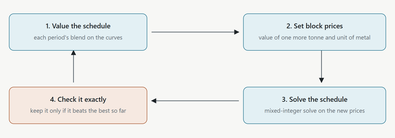
- Value the schedule on the curves. For each period, Resolve calculates the feed blend for new ore and reclaimed stock that share a treatment route. Resolve accounts separately for opening stock with its own recovery assumptions. The curves give recovery, and the run's commercial terms give revenue and royalty.
- Set block prices. Resolve measures how much the period's revenue changes for one more tonne of feed, and for one more unit of contained metal or other assay mass, at that blend. Each block and stockpile lot is priced in each period from its tonnes and assays using those marginal values. The straight-line approximation matches the current blend's value and estimates the effect of small changes nearby.
- Solve the schedule on those prices with every other rule of the case: stope order, benches, capacities, closure and tax.
- Check it exactly. The new schedule is valued on the curves again (step 1). A round that improves on the best schedule so far becomes the new best. The next round uses its prices and starts from that schedule.
The run stops at its round or time limit, when a round does not improve on the best, or when recovery changes fall within the tolerance. It reports the best schedule's value on the curves.
Example: recovery changes the reclaim order
To anonymise the case, this example uses invented figures and a fictional relationship between iron (Fe) grade and zinc (Zn) recovery.
The mill needs 80,000 t of fresh ore and 20,000 t of stockpile reclaim each month. Fresh ore contains 7% iron in month 1 and 3% in month 2. Two accessible stockpile lots of 20,000 t each contain 2% and 8% iron. All ore grades 4% zinc. Both reclaim sequences meet the feed limits and have the same reclaim cost. Iron affects value only through its effect on zinc recovery in this example.
Assume zinc recovery is 85% at 6% iron or less and falls to 80% at 7.2% iron. Each month feeds 4,000 t of contained zinc.
| Reclaim order | Month 1 recovery | Month 2 recovery | Total zinc recovered |
|---|---|---|---|
| Low-iron lot first | 85% | 85% | 6,800 t |
| High-iron lot first | 80% | 85% | 6,600 t |
Taking the low-iron lot first brings month 1 feed down to 6% iron. The high-iron lot can then go into the lower-iron fresh feed in month 2, where the blend is 4% iron. The change in reclaim order recovers 200 t more zinc from the same ore.
The monthly step
The annual rounds price each year's feed as one blend. The monthly step re-plans the plant side month by month on top of a finished annual run.
- Build a monthly case from the annual run. Use months for the years with mill feed, then whole years to the end of the horizon.
- Hold the mining. Each stope and bench is held at the position the annual run reached at each year end, with the annual run's capital and closure year. Inside a year, the timing of mining by month is free within the case's monthly limits.
- Free the plant side. Which ore goes to the plant in which month, and what is stockpiled and reclaimed, is re-optimised, including moving stockpiled ore between years. A fixed annual reclaim commitment can be spread across months by days.
- Price each month on its own blend. The same rounds as above run on the monthly periods. Each month's feed is valued on the curves using its own head grades. The minimum feed threshold scales to each month's share of the year.
- Tax by financial year. An after-tax monthly run taxes each financial year on the sum of its months, with the same terms as the annual run.
Twelve months with identical blends reproduce the annual value on the same recovery curves and commercial terms. A gain from monthly replanning depends on whether the plant can run the proposed campaigns.
Where the method comes from
Sequential (or successive) linear programming was introduced by Griffith and Stewart at Shell Oil in 1961 to optimise refinery processing systems. Replace a curved model by a linear one at the current operating point, solve the linear programme, move to the new point and repeat [1]. A trust region can bound each trial step, keeping it close to the point where the model was linearised [6].
Refinery planning met the same structure in pooling: streams are mixed in a tank, and the pool's quality (sulphur, octane) depends on what goes in. Planners priced each stream at the pool's current quality, solved, recomputed the quality and solved again. The method became known as recursion or distributive recursion. Haverly's 1978 studies showed how it behaves, including that it can settle at a local rather than global optimum [2]. Later work showed that distributive recursion in commercial refinery packages is successive linear programming under a change of variables [3].
| Refinery pooling | Mine scheduling | |
|---|---|---|
| Blended pool | Gasoline or diesel pool in a tank | A period's plant feed |
| Quality that depends on the blend | Sulphur, octane, vapour pressure | Pb, Zn and Ag recoveries from head grades |
| What gets priced | Each crude or intermediate stream | Each block and stockpile lot, by period |
| Linear model solved each pass | Refinery LP | Mixed-integer mine schedule (Gurobi) |
What was adapted for the mine
- Integer schedule. Each pass solves a mixed-integer schedule. It can require stopes to finish once started, select one cut-off design per stope, enforce bench sequencing, buy equipment in whole units and tie site closure to the last mill feed.
- Silver split. Silver reports to two concentrates with separate curves and separate payment terms.
- Stockpiles. Blended stockpile lots and opening stock are priced by period like blocks.
- Thin periods. A period below the minimum feed threshold can take a neighbouring period's recoveries, so that a small tail of feed cannot set the price of everything else.
- After tax. When after-tax NPV is selected, Resolve recalculates income tax using each round’s prices.
- Exact check. Resolve applies the original nonlinear recovery curves to each candidate schedule’s feed blends to recalculate recovered metal and revenue. In an after-tax run, it recomputes income tax from the resulting annual cash flows. It retains the schedule with the highest recalculated NPV found. The MIP gap applies to the linear model solved in each round. A global bound on the nonlinear scheduling problem requires a separate calculation.
How it can be checked
Each run's report page has a Recovery workbook download. It lists every period's feed blend with the curve formulas live in Excel. Head grades, recoveries, recovered metal, concentrates and revenue appear beside the run's own figures.
References
- Griffith, R.E. and Stewart, R.A. (1961). A nonlinear programming technique for the optimization of continuous processing systems. Management Science 7(4), 379–392. Shell Oil, Houston. doi:10.1287/mnsc.7.4.379
- Haverly, C.A. (1978). Studies of the behavior of recursion for the pooling problem. ACM SIGMAP Bulletin, pp. 19–28. Original paper.
- Zhang, W.-Y. et al. (2024). Distributed Recursion Revisited. arXiv:2411.09554.
- Campos, P. H. A. et al. (2022). Geometallurgy-oriented mine scheduling considering volume support and non-additivity. Mining Technology 131(1), 1–11. doi:10.1080/25726668.2021.1963607.
- Chanda, E. K. C. and Dagdelen, K. (1995). Optimal blending of mine production using goal programming and interactive graphics systems. International Journal of Surface Mining, Reclamation and Environment 9(4), 203–208. doi:10.1080/09208119508964748.
- Byrd, R. H. et al. (2005). On the convergence of successive linear-quadratic programming algorithms. SIAM Journal on Optimization 16(2), 471–489. doi:10.1137/S1052623403426532.